Image Sorting and Composition Assessment Part 1 - Online Learning
Approaching photo quality assessment from Machine Learning point of view
- Image Quality Assessment overview
- Lifelong Learning (LL)
- Types of OL/CL algorithm
- Learning without Forgetting
- SequeL
Image Quality Assessment overview
Processing of 2D images are one of the most robust fields within Machine Learning due to high availability of the data. Image quality assessment (IQA) for 2D images is an important area within 2D image processing, and it has many practical applications, one being Photo culling. Photo Culling is a tedious, time-consuming process through which photographers select the best few images from a photo shoot for editing and finally delivering to clients. Photographers take thousands of photo in a single event, and they often manually screen photos one by one, spending hours of effort. Criteria that photographers look for is:
Closed eyes
Noise level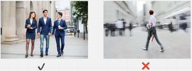
Near duplicate images
Proper light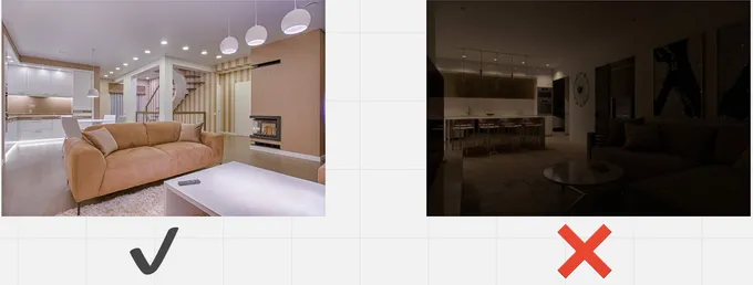
Rule of thirds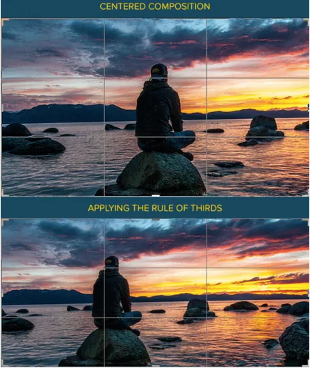
Poses, emotion
Machine learning and IQA
IQA is definitely one of the areas where Machine Learning algorithms can excel at. However, there are many criterias (defined above) that it must fulfill, and the biggest hurdle is that because every photographers have different preferences, you cannot expect one pretrained model to satisfy all the end users. We should implement Continual Learning (CL) process, so that we do not have to retrain entire pipeline of models from scratch. When the end user performs his own version of the culling process based on the suggestions of the pretrained model, this should become the new stream of data for CL training. The original IQA model should be tuned according to this new data, with the aim to minimize training time and the catastrophic forgetting, where the model forgets what it learned before the CL process began.
Now, we need to think about the architecture of this entire pipeline. First, it may be difficult to combine IQA and near-duplicate detevction (NDD) models together. Intuitively, a NDD model should break down the images into N set of images, and within each set, IQA will determine the quality of images. And there must be CL algorithm on top of everything. Ideally, NDD and IQA both should be continuously trainable, if not, at least the IQA portion of the pipeline should be trainable.
Another thing to consider is EXIF data. EXIF (Exchangeable Image File Format) files store important data about photographs. Almost all digital cameras create these data files each time you snap a new picture. An EXIF file holds all the information about the image itself — such as the exposure level, where you took the photo, and any settings you used. Apart from the photo itself, EXIF data could have important details for NDD and IQA. We must see if there is any improvement in the result when we incorporate the EXIF data. It could be totally unnecessary, just making network heavy. But it could prove to be useful as well.
Now, in terms of the representation of the architecture, something like below could make sense: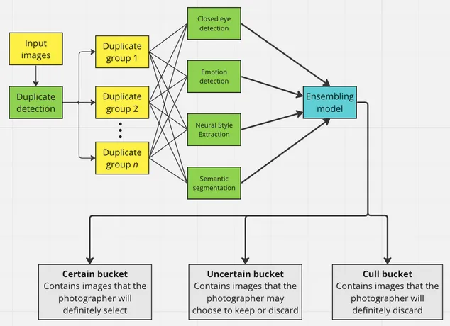
NDD and IQA, I do already have some idea as to how they would work even before doing proper research, but the idea of continuous learning is very vague to me. How are these supposed to be implemented? Does it work on any architecture? What are the limitations?
I feel like it would only make sense for me to look into IQA and NDD closely after having better grasp of CL. Therefore, for the first part of the post, I will checkout Continous Learning.
Lifelong Learning (LL)
If you think about how humans learn, We always retain the knowledge learned in the past and use it to help future learning and problem solving. When faced with a new problem or a new environment, we can adapt our past knowledge to deal with the new situation and also learn from it. The author of Lifelong Machine Learning defines the process to imitate this human learning process and capability as Lifelong learning (LL), and states terms like Online learning and continual learning are subsets of LL.
Online Learning overview
What is Online Learning exactly? Online learning (OL), is a learning paradigm where the training data points arrive in a sequential order. This could be because the entire data is not available yet, due to various reasons like annotations being too expensive, or for cases like us, where we need the users to generate these data.
When a new data point arrives, the existing model is quickly updated to produce the best model so far. In online learning, if whenever a new data point arrives re-training using all the available data is performed, it will be too expensive. It becomes impossible when the model size is big. Furthermore, during re-training, the model being used could already out of date. Thus, online learning methods are typically memory and run-time efficient due to the latency requirement in a real-world scenario.
Much of the online learning research focuses on one domain/task. Objective is to learn more efficiently with the data arriving incrementally. LL, on the other hand, aims to learn from a sequence of different tasks, retain the knowledge learned so far, and use the knowledge to help future task learning. Online learning does not do any of these
Continual learning overview
The concept of OL is simple. The sequence of data gets unlocked in every stage, and the training is performed sequentially to make model more robust. Continual learning is also quite similar, but it is more sophisticated. It needs to learn various new tasks incrementally while sharing paramters with old ones, without forgetting.
Continuous learning is generally divided into three categories: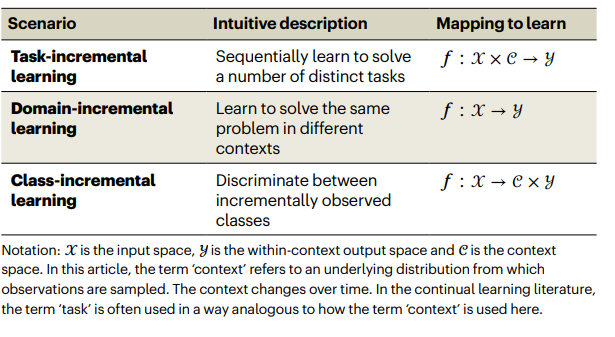
Task Incremental learning
Let’s look at the first scenario. This scenario is best described as the case where an algorithm must incrementally learn a set of distinct tasks. Often times, this task identity is explicit, and it does not require seperate network. If the network requires completely different task (e.g Classification vs Object Detection), it would require seperate network and weights, And there will be no forgetting at all
The challenge with task-incremental learning, therefore, is not—or should not be—to simply prevent catastrophic forgetting, but rather to find effective ways to share learned representations across tasks, to optimize the trade-off between performance and computational complexity and to use information learned in one task to improve performance on other tasks
Now assume this scenario for MNIST: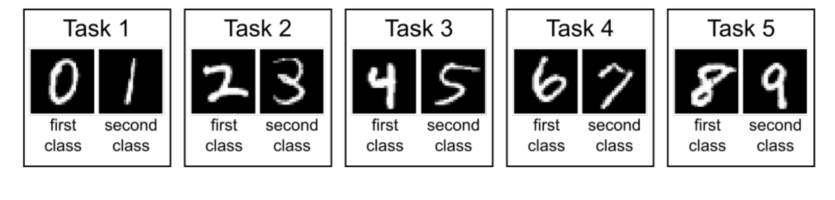
So the objective here would be to ensure that learning Task N would make learning of Task N+1 easier, and for above example, even after learning all the way up to Task 5, when we ask to perform classification for Task 1, the model can still perform well without forgetting.
Thus when we have some Input space X and output space Y, with the task context C, we learn to perform \[f : X \times C \rightarrow Y\]
Domain Incremental learning
In this scenario, the structure of the problem is always the same, but the context or input-distribution changes.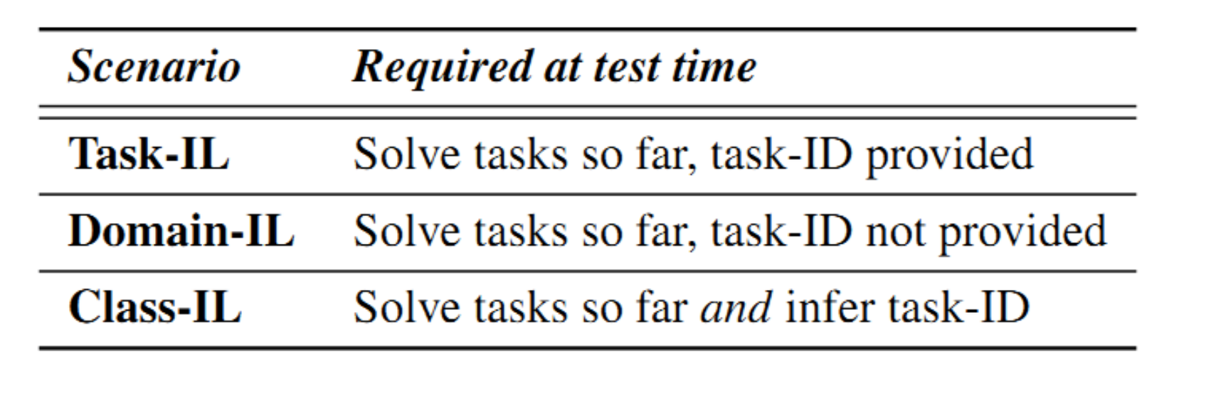
It is similar to Task incremental learning in that every training round n, we expect the model to learn from Dataset n: \[D_n = {(x_i, y_i)}\]
But at the test time, we do not know which “task” it came from. This is probably the most relevant cases for our pipeline. The available labels (classes) will remain the same, and domain will keep on changing. We do not care or want to provide task context. Thus intuitively, this is: \[f : X \rightarrow Y\]
Class Incremental learning
The final scenario is the class incremental learning. This is more popular field of study within continual learning, and most continual learning papers at CVPR were targeted for class incremental learning as well, because this is the area where often times the catastrophic forgetting (CF) happens most significantly. This scenario is best described as the case where an algorithm must incrementally learn to discriminate between a growing number of objects or classes.
Data arrives incrementally as a batch of per-class sets X i.e. (\(X\), \(X^2\), …, \(X^t\) ), where \(X^y\) contains all images from class y. Each round of learning from one batch of classes is considered Task \(T\). At each step \(T\), complete data is only available for new classes \(X\), and the only small number previously learned classes are available as memory buffer. If not using rehearsal technique, the memory buffer is not even available. The algorithm must map out global label space, and at testing time, it would not have any idea of which step the data came from.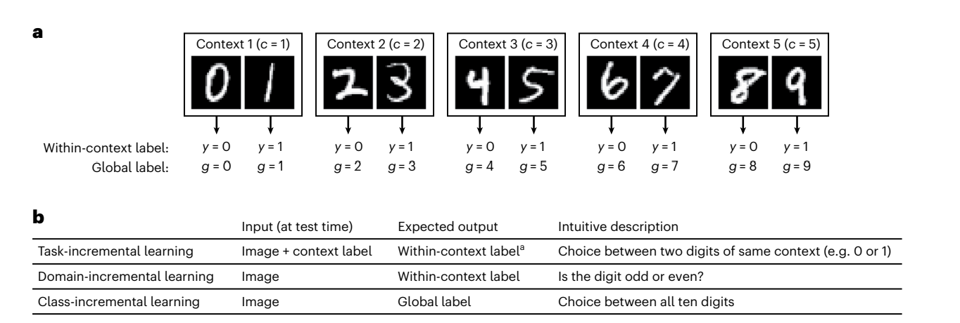
And this is out of scope of this research. Why?
The new data that users will be adding over time will span across multiple classes, and a lot of them will be from previously seen classes. The strict protocol of class-incremental learning would not make sense.
Single head vs Multi-head evaluation
The system should be able to differentiate the tasks and achieve successful intertask classification without the prior knowledge of the task identifier (i.e. which task current data belongs to). In the case of single-head, the neural network output should consist of all the classes seen so far, so the output should be evaluated in the global scale. In contrast, multi-head evaluation only deals with intra-task classification where the network output only consists of a subset of all the classes.
For MNIST, say that the dataset is broken down by classes into 5 tasks, where we have [{0,1}....{8,9}]
In multi-head setting, we would know the ask number (let’s say Task 5), and we would only be making prediction b/w the subset {8,9}. Typically Task-incremental learning will fall under this.
In single-head setting, evaluation will be down across all ten classes, so {0…9}. Typically domain incremental and class incremental learning will fall under this.
Types of OL/CL algorithm
My conclusion after research is that although some authors make clear distinctions b/w Life long learning, Online learning and Continual Learning as most use them interchaneably. Regardless of being OL or CL, these properties are shared:
- Online model parameter adaptation: How to update the model parameters with the new data?
- Concept drift: How to deal with data when the data distribution changes over time?
- The stability-plasticity dilemma: If the model is too stable, it can’t learn from the new data. When the model is too plastic, it forgets knowledge learned from the old data. How to balance these two?
- Adaptive model complexity and meta-parameters: The presence of concept drift or introducing a new class of data might necessitate updating and increasing model complexity against limited system resources

So the main challenge, as everyone agrees, is to make model plastic enough to learn due data, but stable enough to not forget the previously gained knowledge. Finding this balance is the key to online learning. Now we look at some of the methods.
Replay methods
Replay methods are based on repeatedly exposing the model to the new data and data on which it has been already trained on. New data is combined with sampled old data, and can be used for rehearsal (thus retaining training data of old sub-tasks) or as constraint generators. If the retained samples are used for rehearsal, they are trained together with samples of the current sub-task. If not, they are used directly to characterize valid gradients.
The main differences b/w replay methods exists in the following:
- How examples are picked and stored
- How examples are replayed
- How examples update the weights
Drawbacks
The storage cost would go up linearly with the tasks. Yes, we are sampling from older data, but as round progresses, the storage of older data would be required to increase.
Relevant papers
- An Investigation of Replay-based Approaches for Continual Learning
- Sample Condensation in Online Continual Learning
- Measuring Catastrophic Forgetting in Neural Networks
- Mitigating Catastrophic Forgetting in Deep Learning in a Streaming Setting Using Historical Summary
CVPR
Parameter Isolation methods
Parameter isolation methods try to assign certain neurons or network resources to a single sub-task. Dynamic architectures row, e.g., with the number of tasks, so for each new sub-task new neurons are added to the network, which do not interfere with previously learned representations. This is not relevant to us since we do not want to add additional tasks to the network.
Regularization methods
Regularization methods work by adding additional terms to the loss function. Parameter regularization methods study the effect of neural network weight changes on task losses and limit the movement of important ones, so that you do not deviate too much from what you learned previously.
Relevant papers
- Overcoming catastrophic forgetting in neural networks
- Riemannian Walk for Incremental Learning: Understanding Forgetting and Intransigence
CVPR
Knowledge Distillation methods
Originally designed to transfer the learned knowledge of larger network (teacher) to a smaller one (student), knowledge distillation methods have been adapted to reduce activation and feature drift in continual learning. Unlike regularization methods that regularize the weights, KD methods regularize the network intermediate outputs.
Relevant papers
CVPR
Learning without Forgetting
Now that we have some general idea of how incremental learning works, let’s look at a paper in depth. Learning without Forgetting released in 2017 is probably one of the earliest and most famous work done in this field. This may not be perfectly suitable for our scenario where label space b/w previous task overlaps and may or may not contain novel class, but it is still important in the sense that you can understand general mechanism.
SequeL
This is based on this CVPR paper. SequeL is a flexible and extensible library for Continual Learning that supports both PyTorch and JAX frameworks. SequeL provides a unified interface for a wide range of Continual Learning algorithms, including regularization- based approaches, replay-based approaches, and hybrid approaches.